What makes microservices instrumentation different than instrumentation of monolithic systems?

Observability activities involve measuring, collecting, and analyzing various diagnostics signals from a system. These signals may include metrics, traces, logs, events, profiles and more. In monolithic systems, the scope is a single process. A user request comes in and goes out from a service. Diagnostic data is collected in the scope of a single process.

When we first started to build large-scale microservices systems, some practices from the monolithic systems didn’t scale. A typical problem is to collect signals and being able to tell if we are meeting SLOs between them. Unlike the monolithic systems, nothing is owned end-to-end by a single team. Various teams build various parts of the system and agree to meet on an SLO.

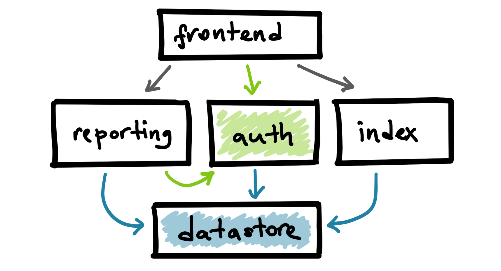
Authentication service depends on the datastore and ask their team to meet a certain SLO. Similarly, reporting and indexing services depend on datastore.

In microservices architectures, it is likely that some services will be a common dependency for a lot of teams. Some examples of these services are authentication and storage that everyone needs and ends up depending on. On the other hand, more particularly, expectations from services vary. Authentication and indexing services might have wildly different requirements from the datastore service. Datastore service needs to understand the individual impact of all of these different services.

This is why adding more dimensions to the collected data became important. We call these dimensions labels or tags. Labels are key/value pairs we attach to the recording signal, some example labels are the RPC name, originator service name, etc. Labels are what you want to breakdown your observability data with. Once we collect the diagnostics signal with enough dimensions, we can create interesting analysis reports and alerts. Some examples:

• Give me the datastore request latency for RPCs originated at the auth service.
• Give me the traces for rpc.method = “datastore.Query”.

The datastore service is decoupled from the other services and doesn’t know much about the others. So it is not possible for the datastore service to add fine grained labels that can reflect all the dimensions user want to see when they break down the collected diagnostics data.

The solution to this problem is to produce the labels at the upper-level services that calls into the lower-level services. After producing these labels, we will propagate them on the wire as a part of the RPC. The datastore service can enrich the incoming labels with additional information it already knows (such as the incoming RPC name) and record the diagnostics data with the enriched labels.

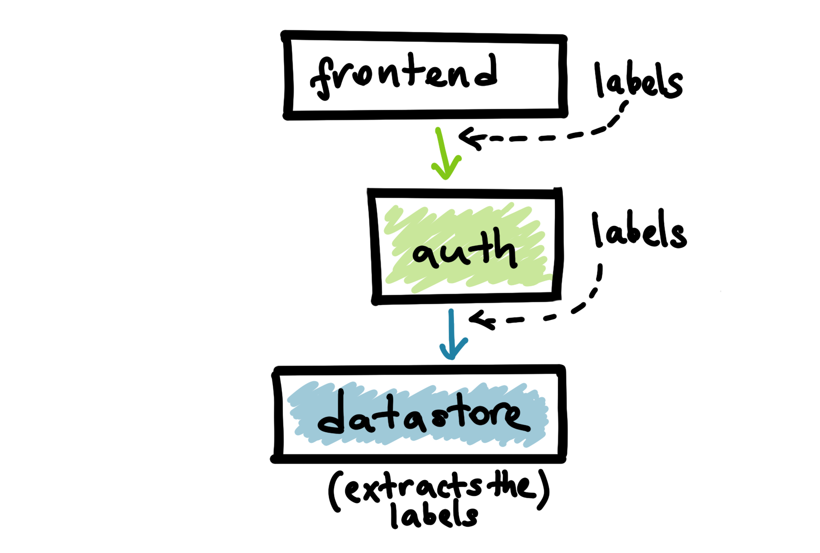
Context is the general concept to propagate various key/values among the services in distributed systems. We use the context to propagate the diagnostics related key/values in our systems. The receiving endpoint extracts the labels and keep propagating them if it needs to make more RPCs in order to respond to the incoming call.

Above high-level services such as the frontend and auth can produce or modify labels that will be used when datastore is recording metrics or logs. For example, datastore metrics can differentiate calls coming from a Web or a mobile client via labels provided at the frontend service.

This is how we have fine grained dimensions at the lower ends of the stack regardless of how many layers of services there are until a call is received at the lowest end.

We can then use observability signals to answer some of the critical questions such as:

• Is the datastore team meeting their SLOs for service X?
• What’s the impact of service X on the datastore service?
• How much do we need to scale up a service if service X grows 10%?

Propagating labels and collecting the diagnostics data are opening a lot of new ways to consume the observability signals in distributed systems. This is how your teams understand the impact of services all across the stack even if they don’t know much about the internals of each other’s services.

Non-uniform memory access (NUMA) is an approach to optimize memory access time in multi-processor architectures. In NUMA architectures, processors can access to the memory chips near them instead of going to the physically distant ones.

In the distant past CPUs generally ran slower than the memory. Today, CPUs are quite faster than the memory they use. This became a problem because processors constantly started to wait for data to be retrieved from the memory. As a result of such data starvation problems, for example, CPU caches became a popular addition to modern computer architecture.

With multi processors architectures, the data starvation problem became worse. Only one processor can access the memory at a time. With multiple processors trying to access to the same memory chip resulted in further wait times for the processors.

NUMA is an architectural design and a set of capabilities trying to address problems such as:

• Data-intensive situations where processors are starving for data.
• Multi-processor architectures where processors non-optimally race for memory access.
• Architectures with large number of processors where physical distance to memory is a problem.

Nodes

NUMA architectures consist of an array of processors closely located to a memory. Processors can also access the remote memory but the access is slower.

In NUMA, processors are grouped together with local memory. These groups are called NUMA nodes. Almost all modern processors also contains a non-shared memory structure, CPU caches. Access to the caches are the fastest, but shared memory is required if data needs to be shared. In shared cases, access to the local memory is the fastest. Processors also have access to remote memory. The difference is that accessing remote memory is slower because the interconnect is slower.

NUMA architectures provide APIs for the users to set fine-tuned affinities. The main way how this works is to allocate memory for a thread on its local node. Then, make the thread running in the same node. This will allow the optimal data access latency for memory.

Linux users might be familiar with sched_setaffinity(2) which allows its users to lock a thread on a specific processor. Think about NUMA APIs as a way to lock a thread to a specific set of processors and memory. Even if the thread is preempted, it will only start rerunning on a specific node where data locality is optimal.

NUMA in Linux

Linux has NUMA support for a while. NUMA supports provides tools, syscalls and libraries.

numactl allows to set affinities and gather information about your existing system. To gather information about the NUMA nodes, run:

$ numactl --hardware

You can set affinities of a process you are launching. The following will set the CPU node affinity of the launching process to node 0 and will only allocate from 0.

$ numactl --cpubind=0 --membind=0 <cmd>

You can allocate memory preferable on the given node. It will still allocate memory in other nodes if memory can't be allocated on the preferred node:

$ numactl --preferred=0 <cmd>

You can launch a new process to allocate always from the local memory:

$ numactl --localalloc <cmd>

You can selectively only execute on the given CPUs. In the following case, the new process will be executed either on processor 0, 1, 2, 5 or 6:

$ numactl --physcpubind=0-2,5-6 <cmd>

See numactl(8) for the full list of capabilities. Linux kernel supports NUMA architectures by providing some syscalls. From user programs, you can also call the syscalls. Alternatively, numa library provides an API for the same capabilities.

Optimizations

Your programs may need NUMA:

• If it's clear from the nature of the problem that memory/processor affinity is needed.
• If you have been analyzing CPU migration patterns and locking a thread to a node can improve the performance.

Some of the following tools could be useful diagnosing the need for optimizations.

numastat(8) displays some hits or misses per node. You can see if memory is allocated as intended on the prefered nodes. You can also see how often memory is allocated on local vs remote.

numatop allows you to inspect the local vs remote memory access stats of the running processes.

You can see the distance between nodes via numactl --hardware to avoid allocating from distant nodes. This will allow you to optimize to avoid the overhead of the interconnect.

If you need to further analyze thread scheduling and migration patterns, tracing tools such as Schedviz might be useful to visualize kernel scheduling decisions.

One more thing…

Recently, on the Go Time podcast, I briefly mentioned how I'm directly calling into libnuma from Go programs for NUMA affinity. I think, everyone was thinking I was joking. In Go, runtime scheduler doesn't allow you to have precise control or doesn't expose the underlying processor/architecture. If you are running highly CPU intensive goroutines with strict memory access requirements, NUMA bindings might be an option.

One thing you need to make sure is to lock the OS thread, so the goroutine is kept being scheduled to run on the same OS thread which can set its affinity via NUMA APIs.

DON'T TRY THIS HOME (unless you know what you are doing):

import "github.com/rakyll/go-numa"

func main() {
	if !numa.IsAvailable() {
		log.Fatalln("NUMA is not available on this machine.")
	}

	// Make sure the underlying OS thread
	// doesn't change because NUMA can only
	// lock the OS thread to a specific node.
	runtime.LockOSThread()

	// Runs the current goroutine always in node 0.
	numa.SetPreferred(0)
    // Allocates from the node's local memory.
    numa.SetLocalAlloc()

	// Do work in this goroutine...
}

Please don't use this if you are 100% sure what you are doing. Otherwise, it will limit the Go scheduler and your programs will see a significant performance penalty.

Note: This article mentions Google Cloud components.

If you are a cloud user, you probably have seen how unconventional storage options can get. This is even true for disks you access from your virtual machines. There are not many ongoing conversations or references about the underlying details of core infrastructure. One such lacking conversation is how fundamentally Google Persistent Disks and replication works.

Disks as services

Persistent disks are NOT local disks attached to the physical machines. Persistent disks are networking services and are attached to your VMs as network block devices. When you read or write from a persistent disk, data is transmitted over the network.

Persistent disks heavily rely on Google’s file system called Colossus. Colossus is a distributed block storage system that is serving most of the storage needs at Google. Persistent disk drivers automatically encrypt your data on the VM before it goes out of your VM and transmitted on the network. Then, Colossus persists the data. Upon a read, the driver decrypts the incoming data.

Having disks as a service is useful in various cases:

• Resizing the disks on-the-fly becomes easier. Without stopping a VM, you can increase the disk size (even abnormally).
• Attaching and detaching disks becomes trivial. Given disks and VMs don’t have to share the same lifecycle or to be co-located, it is possible to stop a VM and boot another one with its disk.
• High availability features like replication becomes easier. The disk driver can hide replication details and provide automatic write-time replication.

Disk latency

Users often wonder the latency overhead of having disks as a networking service. There are various benchmarking tools available. Below, there are a few reads of 4 KiB blocks from a persistent disk:

$ ioping -c 5 /dev/sda1
4 KiB <<< /dev/sda1 (block device 10.00 GiB): time=293.7 us (warmup)
4 KiB <<< /dev/sda1 (block device 10.00 GiB): time=330.0 us
4 KiB <<< /dev/sda1 (block device 10.00 GiB): time=278.1 us
4 KiB <<< /dev/sda1 (block device 10.00 GiB): time=307.7 us
4 KiB <<< /dev/sda1 (block device 10.00 GiB): time=310.1 us
--- /dev/sda1 (block device 10.00 GiB) ioping statistics ---
4 requests completed in 1.23 ms, 16 KiB read, 3.26 k iops, 12.7 MiB/s
generated 5 requests in 4.00 s, 20 KiB, 1 iops, 5.00 KiB/s
min/avg/max/mdev = 278.1 us / 306.5 us / 330.0 us / 18.6 us

GCE also allows attaching local SSDs to virtual machines in cases where you have to avoid a longer roundtrip. If you are running a cache server or running large data processing jobs where there is an intermediate output, local SSDs would be your choice. Unlike persistent disks, data on local SSDs are NOT persistent and will be flushed each time your virtual machine restarts. It is only suitable for the optimization cases. Below, you can see the latency observed from 4 KiB reads from an NVMe SSD:

$ ioping -c 5 /dev/nvme0n1
4 KiB <<< /dev/nvme0n1 (block device 375 GiB): time=245.3 us(warmup)
4 KiB <<< /dev/nvme0n1 (block device 375 GiB): time=252.3 us
4 KiB <<< /dev/nvme0n1 (block device 375 GiB): time=244.8 us
4 KiB <<< /dev/nvme0n1 (block device 375 GiB): time=289.5 us
4 KiB <<< /dev/nvme0n1 (block device 375 GiB): time=219.9 us
--- /dev/nvme0n1 (block device 375 GiB) ioping statistics ---
4 requests completed in 1.01 ms, 16 KiB read, 3.97 k iops, 15.5 MiB/s
generated 5 requests in 4.00 s, 20 KiB, 1 iops, 5.00 KiB/s
min/avg/max/mdev = 219.9 us / 251.6 us / 289.5 us / 25.0 us

Replication

When creating a new disk, you can optionally choose to replicate the disk within region. Persistent disks are replicated for higher availability. Replication happens within a region between two zones.

It is unlikely for a region to fail altogether but zonal failures happen more commonly. Replicating within the region at different zones is a good bet from the availability and disk latency perspective. If both replication zones fail, it is considered a region-wide failure.

In the replicated scenario, the data is available in the local zone (us-west1-a) which is the zone the virtual machine is running in. Then, the data is replicated to another Colossus instance in another zone (us-west1-b). At least one of the zones should be the same zone the VM is running in. Please note that, persistent disk replication is only for the high availability of the disks. Zonal outages may also affect the virtual machines or other components that might cause outage.

Read/write sequences

The heavy work is done by the disk driver in the user VM. As a user, you don’t have to deal with the replication semantics, and can interact with the file system the usual way. The underlying driver handles a sequence for reading and writing.

When a replica falls behind and replication is incomplete, read/writes go through the trusted replica until a reconciliation happens. Otherwise, we are in the full replication mode.

In the full replication mode:

• When writing, a write request tries to write to both replicas and acknowledge when both writes succeed.
• When reading, read request is sent to the local replica at the zone the virtual machine is running in. If the read request times out, another read request is sent to the remote replica.

It is not always obvious to the users that persistent disks are network storage devices. They enable many use cases and functionality in terms of capacity, flexibility and reliability conventional disks cannot provide.

Have you ever launched a new service to production? Have you ever been maintaining a production service? If you answer “yes” to one of these questions, have you been guided during the process? What's good or bad to do in production? And how do you transfer knowledge when new team members want to release production services or take the ownership of existing services?

Most companies end up having organically grown approaches when it comes to production practices. Each team would figure out their tools and best practices themselves with trial-error. This reality often has a real tax not only on the success of the projects but also on engineers.

Trial-error culture creates an environment where finger pointing and blaming is more common. Once these behaviors are common, it becomes harder to learn from mistakes or not to repeat them again.

Successful organizations:

• acknowledge the need of production guidelines
• spend time on researching practices that apply to them
• start having production readiness discussions when designing new systems or components
• enforce production readiness practices

Production readiness involve a “review” process. Reviews can be a checklist or a questionnaire. Reviews can be done manually, automatically or both. Organizations can produce checklist templates rather than a static list of requirements that can be customized based on the needs. By doing so, it is possible to give engineers a way to inherit knowledge but also enough flexibility when it is required.

When to review a service for production readiness?

Production readiness reviews is not only useful right before pushing to production, they can be a protocol when handing off operational responsibilities to a different team or to a new hire. Use reviews when:

• Launching a new production service.
• Handing off the operations of an existing production service to another team such as SRE.
• Handing off the operations of an existing production service to new individuals.
• Preparing oncall support.

Production readiness checklists

A while ago, I published an example checklist for production readiness as an example of what they can cover. Even though the list came to existence when working with Google Cloud customers, it is useful and applicable outside of Google Cloud.

Design and Development

• Have reproducible builds, your build shouldn’t require access to external services and shouldn’t be affected by an outage of an external system.
• Define and set SLOs for your service at design time.
• Document the availability expectations of external services you depend on.
• Avoid single points of failures by not depending on single global resource. Have the resource replicated or have a proper fallback (e.g. hardcoded value) when resource is not available.

Configuration Management

• Static, small and non-secret configuration can be command-line flags. Use a configuration delivery service for everything else.
• Dynamic configuration should have a reasonable fallback in the case of unavailability of the configuration system.
• Development environment configuration shouldn’t inherit from production configuration. This may lead access to production services from development and can cause privacy issues and data leaks.
• Document what can be configured dynamically and explain the fallback behavior if configuration delivery system is not available.

Release Management

• Document all details about your release process. Document how releases affect SLOs (e.g. temporary higher latency due to cache misses).
• Document your canary release process.
• Have a canary analysis plan and setup mechanisms to automatically revert canaries if possible.
• Ensure rollbacks can use the same process that rollouts use.

Observability

• Ensure the collection of metrics that are required by your SLOs are collected and exported from your binaries.
• Make sure client- and server-side of the observability data can be differentiated. This is important to debug issues in production.
• Tune alerts to reduce toil, for example remove alerts triggered by the routine events.
• Include underlying platform metrics in your dashboards. Setup alerting for your external service dependencies.
• Always propagate the incoming trace context. Even if you are not participating in the trace, this will allow lower-level services to debug debug production issues.

Security and Protection

• Make sure all external requests are encrypted.
• Make sure your production projects have proper IAM configuration.
• Use networks within projects to isolate groups of VM instances.
• Use VPN to securely connect remote networks.
• Document and monitor user data access. Ensure that all user data access is logged and audited.
• Ensure debugging endpoints are limited by ACL.
• Sanitize user input. Have payload size restrictions for user input.
• Ensure your service can block incoming traffic selectively per user. This allows to block the abuse cases without impacting other users.
• Avoid external endpoints that triggers a large number of internal fan-outs.

Capacity planning

• Document how your service scales. Examples: number of users, size of incoming payload, number of incoming messages.
• Document resource requirements for your service. Examples: number of dedicated VM instances, number of Spanner instances, specialized hardware such as GPUs or TPUs.
• Document resource constraints: resource type, region, etc.
• Document quota restrictions to create new resources. For example, document the rate limit of GCE API if you are creating new instances via the API.
• Consider having load tests for performance regressions where possible.

Debugging and debugging tools might be irreplaceable to examine the execution flow and the current state of a program. Given it is not always easy to reproduce bugs, being able to debug in production sometimes is a critical benefit. But intercepting a live program in production for debugging purposes is not feasible because it would impact the production system. Conventional diagnostics signals such as logs and traces help to debug programs without impacting the execution flow but they might be limited in terms of reporting the critical variables and don't have capabilities to evaluate new expressions.

Additionally, logs or stacktraces might not be helpful to diagnose problems at all. If a process is crashing consistently without enough diagnostics, it might be hard to pinpoint to the problem without conventionally debugging the program. The difficulty of reproducing production environments lead to the fact it is hard to reproduce the execution flows that are taking place in production.

Debugging production bugs is often challenging it requires reproduction of a similarly orchestrated environment and workload. If the bug is causing any downtime, it is critical for developers/operators to be able to take action without risking cascading failures.

To understand a program at any exact moment, we use core dumps. A core dump is a file that contains the memory dump of a running process and its status. It is primarily used for post-mortem debugging of a program and to understand a program’s state while it is still running with minimal overhead.

Core dumps are not only useful for debugging user-space programs but the state of the kernel when snapshot is taken. We can classify core dumps mainly into two categories:

• Kernel dumps: Core dumps that contain the full or partial memory of the entire system. It is useful to understand the state of the kernel and other programs that might be triggering bugs.
• Platform dumps: Core dumps that contain the memory of a platform, or agent such as JVM.
• User-space dumps: Core dumps that contain the memory dumps of a single user-space process. Useful to investigate user-space problems.

Two strategies are adopted to capture dumps:

• Automatically have a dump upon process crash.
• Have a dump upon receiving SIGSEGV, SIGILL, SIGABRT or similar.

Once obtained, core files can be used with conventional debugging tools (e.g. gdb, lldb) interactively to backtrace and to evaluate expressions. Core dumps can also be sent to a service that generate reports and help you analyze dumps more in scale. Core dumps also can be used to build live debugging tools like Stackdriver Debugger to debug production services with minimal overhead.

Obtaining core dumps might introduce some challenges such as:

• PII: Being able to strip out personally identifiable information (PII) can be critical when debugging actual live production systems.
• Core dump retrieval time: Retrieving core dumps might take a long time depending on the extend of the collection and might introduce additional overhead.
• Core dump size: Depending on the extend of the dump, the core dump file size can get quite large. This presents a challenge when automatically capturing dumps and storing term in the long term in scale.

For further reading on obtaining core dumps, see:

• How to get a core dump for a segfault on Linux
• Capturing JVM core dumps
• Capturing Go core dumps

Benchmarking generally mean producing some measurements from a specific program or workload to typically understand and compare the performance characteristics of the benchmarked workload.

Benchmarks can be useful for:

• Optimizing costly workloads.
• Understanding how the underlying platform impact the cost.

Benchmarking can give you insights about your workload on various dimensions such as CPU cycles spent or memory allocation done for a given task. These measurements (even though they might be coming from idealized environments) might give you some hints about the cost. They may help you to pick the right algorithm or optimize an overwhelmingly expensive workload.

Benchmarking can also give you insights about the underlying runtime, operating system, and hardware. And you might find insights to compare how each of these elements impact your performance even if you don't change the code. You might want to run the same suite of benchmarks on a new hardware to estimate the impact of the new hardware on certain calls.

Benchmarking requires a deep understanding of all layers you depend on. Consider CPU benchmarking. Any aspect below can significantly impact your results:

• Whether the data is available in the CPU cache or not.
• Whether you hit a garbage collection or not.
• Whether compiler has optimized some cases or not.
• Whether there is concurrency or not.
• Whether you are sharing the cores with anything else.
• Whether your cores are virtual or physical.
• Whether the branch detector will do the same thing or not.
• Whether the code you are benchmarking has any side effects or not. Compilers are really good optimizing cases if it has no impact on the global state.

This is why when we talk about benchmarking, it is not good practice to limit ourselves to the user-space code. It can sometimes turn into a detective's job to design and evaluate benchmarks. This is why complicated and long workloads are harder to benchmark reliably. It becomes harder to do the right accounting and figure out whether it is the contention, context switches, caching, garbage collector, compiler optimizations or the user-space code.

Even though microbenchmarks can give some insights, they cannot replicate the situations how the workload is going to perform in production. Replicating an average production environment for microbenchmarking purposes is almost an impossible task. This is why microbenchmarks don't always serve a good starting point if you want to evaluate your production performance.

To conclude, replicating production-like situations is not trivial. Understanding the impact of underlying stack requires a lot of experience and expertise. Designing and evaluating benchmarks are not easy. Examining the production services and understanding the call patterns and pointing out the hot calls may provide better insights about your production. In the future articles, I will cover how we think about performance evaluation in production.

In the recent decade, our systems got complex. Our average production environments consist of many different services (many microservices, storage systems and more) with different deployment and production-maintenance cycles. In most cases, each service is built and maintained by a different team — sometimes by a different company. Teams don’t have much insight into others’ services. The final glue that puts everything together is often a staging environment or sometimes the production itself!

Measuring latency and being able to react to latency issues are getting equally complex as our systems got more complex. This article will help you how to navigate yourself at a latency problem and what you need to put in place to effectively do so.

Latency

So, what is latency? Latency is how long it takes to do something. How long does it take to have a response back? How long does it take to process a message in a queue?

We use latency as one of the core measures to tell whether a system is working as intended end-to-end. On the critical path (in the lifetime of a user request), latency is the core element that contributes to the overall user experience. It also allows us whether we are utilizing our resources as expected or our throughput is less than our trajectory.

Even if you are not engaging with latency measurement, you might be already familiar with various tools on a daily basis that reports latency results. As a daily example, various browser developer tools report the time it takes to make all the requests that make up a web page and report the total time:

Latency is a critical element in the SLOs we set between services. Each team set an SLO for their service (e.g. 50th percentile latency can be 20ms, 90th percentile latency can be 80ms, 99th percentile can be 300ms) and monitor their latency to see if there are any SLO violations. (Watch “SLIs, SLOs, SLAs, oh my!” to learn more about SLOs.)

But how do we systematically collect and analyze request latency in today’s production systems?

We measure latency for each request and primarily use metric collection systems to visualize and trigger auto alerts. Latency collection is unsampled (we collect a latency metric for every request) and is aggregated as a histogram distribution to provide visibility to the higher percentiles.

You can use your choice of collection libraries to collect latency metrics.

Is there unexpected latency?

In order to detect anomalies in latency, we need to first answer what would be considered as expected latency. Every service has different requirements what unexpected latency can be. It is almost impossible to have services with 100% reliability, hence we need to first determine what latency range would give user an experience that they wouldn’t recognize there is a problem.

“For inbox.GetEmails call, 99th percentile request latency should be less than 300ms.” is an example SLO where we set the 99th percentile upper bound for latency for the inbox service’s GetEmails method. There might be requests that took more than 300ms but would not violate the SLO if there are not making to the 99th percentile. You can define your SLOs in a lower or higher percentile. (Watch How NOT to Measure Latency to understand why percentiles matter.)

When an SLO violation occurs, we can automatically trigger alerts and ping the on-call person to take a look. Or you can hear from a customer that they are expecting poor latency and ask you to resolve the issue.

What is the source of latency?

When an alert is triggered or a customer is reaching out to you, an on-call person is expected to take a look. At this point, they know that there is a latency violation or poor experience. We often know what specific service/method it is but no idea the underlying cause. At this point, we can look at the latency distribution heat map for the service/method.

Heat maps visualize latency distribution over time; x-axes is the time and y-axes is the latency bucket the measurement fell into. We recently started to correlate latency distribution buckets with exemplar traces that fits into that bucket. This allows us to find a trace from a particular latency bucket when debugging latency issues. (Watch Resolving Outages Faster With Better Debugging Strategies for more details.)

(*) Each green star represents an exemplar for the bucket. When you click on it, it takes you to the trace exemplar and you can see the distributed trace for one of the calls that fell into that bucket.

A click on a star is taking you to the trace where you can see what has happened in the lifetime of that request more granularly. Traces can navigate us to the underlying issue. It will be possible to identify the case if there is an unexpected outage in one of the services we depend on, or a networking problem or an unlikely latency issue.

Once we examine the trace related to the latency bucket at (1), we see Spanner.Apply call took longer than it should from for this particular trace and there are an additional 40ms spent in the doond.GetDocs for a non-RPC job we don’t have additional information about.

Addressing the latency problem

Metrics and traces can navigate you where the latency is rooted but might not be the primary tool understand the underlying cause of the latency. Poor scheduling, networking problems, bad virtualization, language runtime, computationally expensive code and similar problems might be the possible reasons.

Once we narrowed down the source of the latency to a service and sometimes to a specific process, in order to understand the underlying cause, we look at the host-specific and in-process reasons why latency occurred in the first place. For example, a host-specific signal to look at is the utilization and memory metrics.

If the host is behaving normally and networking is not impacted, we may go and further analyze the in-process sources of latency.

Often, servers are handling a large number of requests and there is no easy way to isolate events happened in the lifetime of a request. Some language runtimes like Go allows us to internally trace runtime events in the lifetime of a request. Tools like runtime tracers are often very expensive and we momentarily enable them in production if we are trying to diagnose a problem. We momentarily enable collection, try to replicate the latency issue. We can see if latency is caused by I/O, blocking or stopping-the-world events triggered by the runtime. If not, we can rule out those possibilities.

And sometimes latency is caused by computationally expensive code. For example, if you roll out a new version that is depending on a new compression library, you may experience higher latency than the usual. Being able to label profiler samples with an RPC name is critical to understand the cost of a particular RPC on your server.

Latency is a critical measure to determine whether our systems are running normally or not. Even though metrics can tell whether there is a latency issue, we need additional signals and tools to analyze the situation further. Being able to correlate diagnostics signals with RPC names, host identifiers and environmental metadata allows us to look at various different signals from a particular problem site.

Cindy Sridharan’s fantastic article on why everyone is not ops makes you rethink of the relationship between your development and operations teams.

At Google, SRE stands for site reliability engineer. Site reliability is about velocity and productivity of our engineers, the performance and reliability of our products, and the health of our code base and production environment. I don’t like to say SRE is the Google’s way of doing ops because SRE is a significant rethink of how we do ops. SRE is a standalone organization and is an independent silo at Google. They maintain large production systems at Google, they are the go-to-team for consultancy about anything production related, they set the best practices, they contribute to infra and tools that makes production easy for our software engineers.

What makes Google SRE significantly different is not just their world-class expertise but the fact that they are optional at Google. Yes, I am not missing negation in the previous sentence. They are optional. When we begin working on a new product/project, the development team owns every aspect. From writing design docs to writing code. From unit tests to integration tests. We go through a large series of reviews from security to privacy to production readiness. We are responsible to deploy our code, monitor it, be on call, and put water on fire when required. We do it all ourselves as if there is no SRE or we are our own SREs.

But how does it work if SRE is optional? Working at Google provides you a whole suite of infrastructure you always take for granted. Networking, storage systems, lock systems, auto scaling and scheduling, naming, configuration, and many more. The infrastructure components are staffed by software engineers and often supported by SRE. On the other hand, SRE is not an organization that helps every team in person but they build reusable best practices and support critical technical infrastructure services making production experience better. SRE culture and best practices are very established at Google. Do you want to deploy a production service that scales to the world? We have infrastructure helps you with that. Do you want to have world-class dashboards? We have that. Do you need a plan and better understanding how you should monitor your code? SRE have solutions and best practices for that. Do you want to roll out a new critical service? SRE provide consultancy for that.

The main idea is that SRE organization is not responsible to support any product at Google. You all get the infra and SRE best practices for free, and deserve part-time and later full-time SRE support by becoming a critical and large-scale product. An average timeline how to get SRE support:

• Build a product, coordinate with the team supports launches, ask for SRE consultancy if required.
• Set an SLO, try to recruit part-time SRE support once you hit the critical scale.
• SRE team will require a list of requirements until your product is suitable for their support. Once you meet their criteria, start adding SRE to your on-call rotation.
• Grow the SRE support by using your headcount as your scale grow. Keep your development team responding to the prod issues part-time, so they still understand what’s going on at prod.
• Downscale the SRE support if your project is shrinking in scale, and finally let your development team own the SRE work if the scale doesn’t require SRE support.

This model gives the SRE organization to focus on solutions that scale rather than investing a lot of time on specific products that are not impactful. The SRE headcount on a team is coming from the development team’s headcount, so the development team would prefer to handle SRE job themselves if they are not large enough to ask for additional help. For complex systems and large-scale infrastructure, SRE is there in person as a part of the team. And as they learn, they also contribute to the infrastructure, tools, and knowledge that are reusable by all of the engineering teams at Google.

But does it make everyone ops? At Google, we probably have access to the world’s finest infrastructure to build large-scale systems. Individual teams never have to care about a lock system, databases or our internal naming service. The internal infrastructure is staffed to work and works well. On the top of that, we have a very established SRE culture and software engineers can think and act as an SRE until it is beyond their scale by just adopting the fundamentals and the existing infrastructure. This model helps the software engineers to have a clear understanding of the operational aspects, and give the SRE team the opportunity to be able to focus on impactful projects in a highly sustainable way. I think the industry needs a breakdown between product and infra engineering and start talking how we staff infra teams and support product development teams with SRE. The “DevOps” conversation is often not complete without this breakdown and assuming everyone is self serving their infra and ops all the times.

It is worth to note that Google also has program that allows software engineers to switch to an SRE role for six months called Mission Control. This program allows software engineers to have more in depth understanding how SRE team operates on large-scale systems. Upon finishing the program, they can take back the knowledge and hands-on expertise to their development teams.